
LiDAR & 3D mapping
LiDAR Laser Sources: Build Around the Required Point Cloud
Lumexis develops compact 1535 nm and 1550 nm pulsed laser sources for civil airborne, mobile, terrestrial, and industrial LiDAR systems. Select the source from the complete transmit, receive, timing, and mapping budget—not from peak power alone.
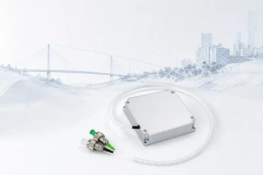
Start with the required point cloud—not the largest peak-power number
Lumexis develops compact 1535 nm and 1550 nm pulsed laser sources for airborne, mobile, terrestrial and industrial LiDAR. Our platform combines nanosecond pulses, externally controlled timing, fiber delivery and compact packaging to help system teams build repeatable 3D measurement around a stable optical source.
A LiDAR laser source should be selected from the final measurement requirement backward. Before comparing models, define:
- the surface and reflectivity range;
- the required operating distance and return margin;
- platform speed, altitude or stand-off distance;
- scanner pattern, field of view and angular sampling;
- required points per second and ground-point spacing;
- range precision and absolute mapping accuracy;
- detector, receiver aperture and optical bandwidth;
- electrical, thermal, mechanical and timing interfaces.
Peak power, pulse width and repetition rate matter, but none of them alone specifies range, point density or mapping accuracy. The right source is the one that closes the complete transmit–receive–timing budget while fitting the host platform.
Lumexis source families for this solution
- 1535 nm and 1550 nm pulsed fiber laser sources for high-rate scanning and dense 3D acquisition.
- 1535 nm erbium-glass laser sources for compact, lower-rate transmitters and selected low-rate sensing architectures.
- Integrated laser rangefinder modules when the system needs a sparse distance channel rather than a raw laser source.
Fast selection rule: Start with pulsed fiber lasers when the scanner needs tens of thousands to millions of emitted pulses per second. Consider erbium-glass sources when compact pulse generation and lower repetition rates are more important than dense point acquisition. Choose an integrated rangefinder module when the host needs distance data, not a transmitter subsystem.
Match the application before matching the laser
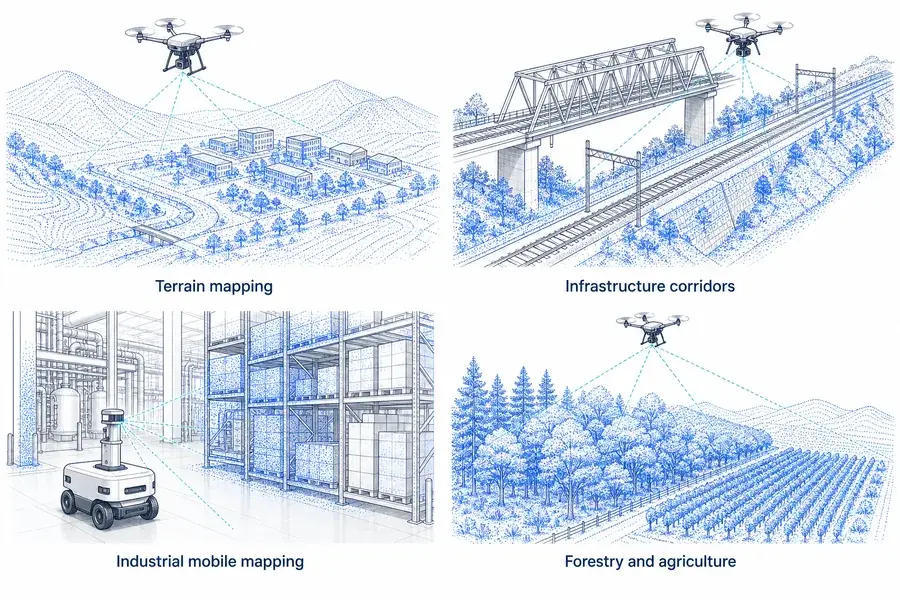
Application fit
Match the optical source to the real measurement task
Four LiDAR application classes: terrain mapping, infrastructure corridors, industrial mobile mapping, and forestry and agriculture
Terrain and topographic mapping
Airborne and uncrewed-platform mapping converts range measurements into georeferenced elevation points. The laser must support the desired along-track and cross-track sampling without creating excessive ambiguity, power draw or thermal load. A compact 1.5 µm pulsed fiber laser is a strong starting point for topographic mapping where the receiver is designed around InGaAs detection.
Infrastructure corridors
Rail, road, bridge, power-line and utility-corridor surveys combine vehicle motion with rapid scanning. Here, reliable trigger behavior, stable pulse timing and mechanical integration can be as important as raw peak power. Higher pulse rates can add samples along narrow assets, but the final point spacing still depends on vehicle speed, scan pattern, field of view and overlap.
Industrial and mobile 3D measurement
Mobile robots, automated inspection platforms and industrial scanners often work at shorter distances but demand compact packaging, predictable synchronization and low integration overhead. A laser with more peak power than the receiver can use may add thermal and electrical burden without improving the final data.
Forestry, agriculture and environmental sensing
Vegetation and uneven natural surfaces produce distributed, multi-level returns. Pulse waveform, receiver bandwidth and processing determine whether the system separates canopy, branches and ground. A short optical pulse helps preserve temporal detail, but vegetation penetration is a complete system property—not a laser-source specification.
Remote infrastructure monitoring
Terrestrial and fixed-position scanners can measure stockpiles, slopes, facades and structural change. These systems may trade platform weight for larger apertures, tighter thermal control or longer dwell time. The source should therefore be chosen for the instrument architecture rather than copied from an airborne design.
Where this solution is not the natural starting point
Clear application boundaries save engineering time:
- Bathymetric mapping: water-penetrating bathymetric LiDAR commonly uses green wavelengths. A 1.5 µm source is intended for topographic and surface-return architectures, not as a direct substitute for a bathymetric transmitter.
- A complete mapping payload: a laser source creates an optical pulse. It does not provide scanning, return detection, GNSS/INS data, point-cloud generation or calibration by itself.
- Coherent wind measurement: Doppler wind LiDAR has different linewidth, coherence and receiver requirements from direct time-of-flight 3D mapping.
- All-weather certainty: fog, cloud, rain, dust and wet or dark surfaces change propagation and return strength. Wavelength choice cannot remove the need for environmental validation.
Choose the correct product boundary
| What the host system needs | Recommended Lumexis starting point | Why |
|---|---|---|
| A high-rate optical pulse train for a scanning LiDAR | 1535/1550 nm pulsed fiber laser | Adjustable high repetition rate, nanosecond pulses, external trigger and fiber delivery |
| A compact, lower-rate transmitter for selected sensing instruments | 1535 nm erbium-glass laser source | Compact source architecture with discrete pulse-energy options |
| Distance values from an integrated channel | 1535 nm laser rangefinder module | Transmit, receive and ranging electronics are already combined |
| A complete georeferenced point cloud | Laser source plus scanner, receiver, timing electronics and navigation sensors | Range must be combined with look direction, position, attitude and calibration |
This distinction prevents a common procurement mismatch. A pulsed laser source is not a rangefinder, and a rangefinder is not a mapping payload. Lumexis can support source selection and interface matching, while the system integrator owns the full scanner, receiver, navigation and processing architecture.
Lumexis pulsed fiber laser platform
The following table is for first-pass matching. Final values and interfaces should be confirmed for the selected operating point and production configuration.
| Model | Wavelength | Peak-power class* | Repetition-rate range | Pulse width | Average-power class | Supply | Envelope | Operating temperature |
|---|---|---|---|---|---|---|---|---|
| 1535-LXMC1.2kw | 1535 nm | 1.2 kW | 100–2000 kHz | 2.5–3.5 ns | 1.2 W | 9–13 V | 55 × 55 × 16 mm | −40 to +75 °C |
| 1550-LXMC1.6kw | 1550 nm | 1.6 kW | 100–2000 kHz | 2.5–3.5 ns | 2.1 W | 9–13 V | 50 × 70 × 19 mm | −40 to +75 °C |
| 1550-LXMC3kw | 1550 nm | 3 kW | 50–2000 kHz | 3–5 ns | 2.0 W | 9–13 V | 50 × 70 × 19 mm | −40 to +75 °C |
*Peak power is operating-point dependent. It must not be assumed to remain constant across the full repetition-rate range.
A practical first-pass match
- Choose 1535-LXMC1.2kw when the design prioritizes a square 55 mm footprint, 1535 nm operation and pulse rates from 100 kHz to 2 MHz.
- Choose 1550-LXMC1.6kw when the receiver is centered at 1550 nm and the system benefits from a higher average-power class within a 50 × 70 mm package.
- Choose 1550-LXMC3kw when more return margin per pulse is required and the wider 3–5 ns pulse is compatible with the timing and spatial-resolution budget.
1535 nm or 1550 nm?
Both wavelengths sit within the sensitivity range of common InGaAs receivers, but the final choice should be made at system level. Check detector responsivity at the exact wavelength, interference-filter availability, fiber and coating losses, atmospheric conditions, supply-chain preference and any wavelength-specific compliance work. A 15 nm difference does not replace a link-budget calculation.
How a laser pulse becomes a georeferenced 3D point
System architecture
Review the complete optical and measurement chain
LiDAR system chain from pulsed laser source through transmit optics, scanner, surface return, InGaAs detector and timing electronics to a georeferenced point cloud
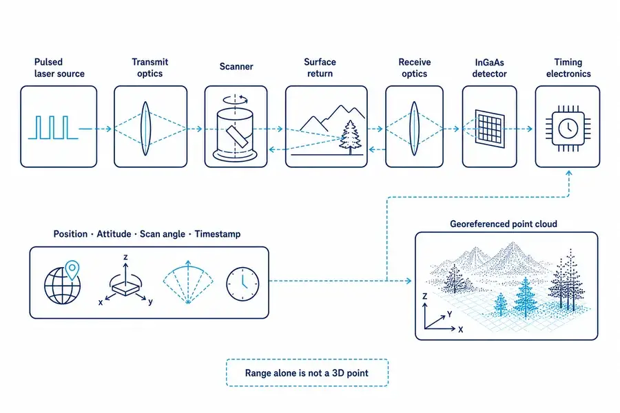
In direct time-of-flight LiDAR, the instrument measures the delay between pulse transmission and return detection:
R = cΔt / 2
where (R) is range, (c) is the speed of light and (Δ t) is the round-trip time.
Range is only one part of a 3D point. The mapping system also needs the scanner look direction, sensor position, platform attitude and a common timestamp. A simplified transformation is:
psurface = psensor + Rulook
The production calculation also includes lever-arm offsets, boresight alignment, coordinate transforms, timing offsets and calibration terms. This is why excellent single-shot range precision can coexist with poor absolute point-cloud accuracy if the navigation or alignment chain is weak.
Four laser parameters that must be evaluated together
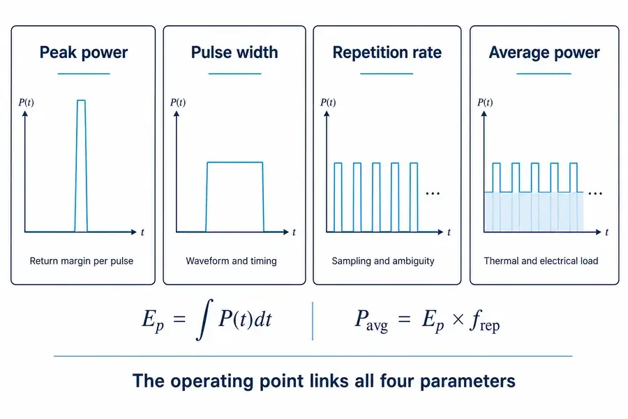
Parameter interaction
Evaluate coupled parameters at the operating point
Engineering diagram explaining how peak power, pulse width, repetition rate and average power influence a pulsed LiDAR system
1. Peak power: return margin per pulse
Higher peak power can increase the photons launched during a short pulse and improve return margin, but only within the limits of the transmit optics, receiver, available pulse energy and operating point. It is not a direct range specification.
The received signal also depends on:
- transmit optical efficiency and beam divergence;
- illuminated spot size at distance;
- surface reflectivity and orientation;
- atmospheric transmission;
- receive-aperture area and field of view;
- filter bandwidth and detector responsivity;
- detector noise, background light and decision threshold.
Comparing two sources by peak power alone is therefore incomplete.
2. Pulse width: waveform and timing
A shorter pulse can support finer temporal discrimination, but the usable range precision also depends on detector bandwidth, signal-to-noise ratio, timing electronics, threshold behavior and the estimation algorithm. Real pulses are not perfect rectangles, so specify how pulse width and peak power are measured.
For an ideal rectangular pulse:
Ep ≈ Ppeakτp
A 1.2 kW, 3 ns ideal rectangular pulse corresponds to approximately 3.6 µJ. A 3 kW, 3 ns pulse corresponds to approximately 9 µJ. These are explanatory calculations, not guaranteed product pulse energies: the actual value is the integral of the measured waveform.
3. Repetition rate: sampling and ambiguity
More emitted pulses can support more measurements per second, but only if the receiver, timing electronics, scanner and processor can accept them. Higher repetition rate also shortens the time before the next pulse and can create pulse-to-return association problems.
For identical, uncoded pulses, a useful first-pass limit is:
Runamb ≈ c / (2frep)
| Pulse repetition rate | Simple first-pass unambiguous range |
|---|---|
| 100 kHz | approximately 1,499 m |
| 500 kHz | approximately 300 m |
| 2 MHz | approximately 75 m |
This table is not a product range claim. Gating, coding, staggered pulse timing, scan context and signal processing can manage ambiguity, but they must be designed into the system.
4. Average power: electrical and thermal reality
Average optical power connects pulse energy and repetition rate:
Pavg = Epfrep
At high pulse rates, average power, conversion efficiency and operating mode drive electrical demand and heat generation. The highest peak-power class may not be available at the maximum repetition rate. Ask for an operating-point map or confirm the required combination of pulse rate, peak power, pulse width and temperature before freezing the design.
Point rate is not point density—and neither is accuracy
These terms are often compressed into a single marketing number, but they describe different things:
- Pulse repetition rate is how often the source emits.
- Measurement rate is how many valid range measurements the receiver produces.
- Point rate is how many points enter the data stream after detection and filtering.
- Point density is the spatial distribution of accepted points over a surface.
- Accuracy is how closely those point coordinates represent their true positions.
For a simple single-return system, valid point rate cannot exceed the accepted measurement rate. Multi-return processing can create several points from one transmitted pulse, while missed detections can reduce the result below the emitted-pulse rate.
Point density then depends on point rate, platform speed, altitude or stand-off distance, scan frequency, field of view, line spacing, overlap and surface visibility. Doubling laser repetition rate does not necessarily double uniform ground density.
Mapping accuracy is a complete calibration chain
Accuracy chain
Treat accuracy as a complete calibration result
LiDAR mapping accuracy chain showing range timing, scanner angle, GNSS position, IMU attitude, lever arm, boresight and clock alignment
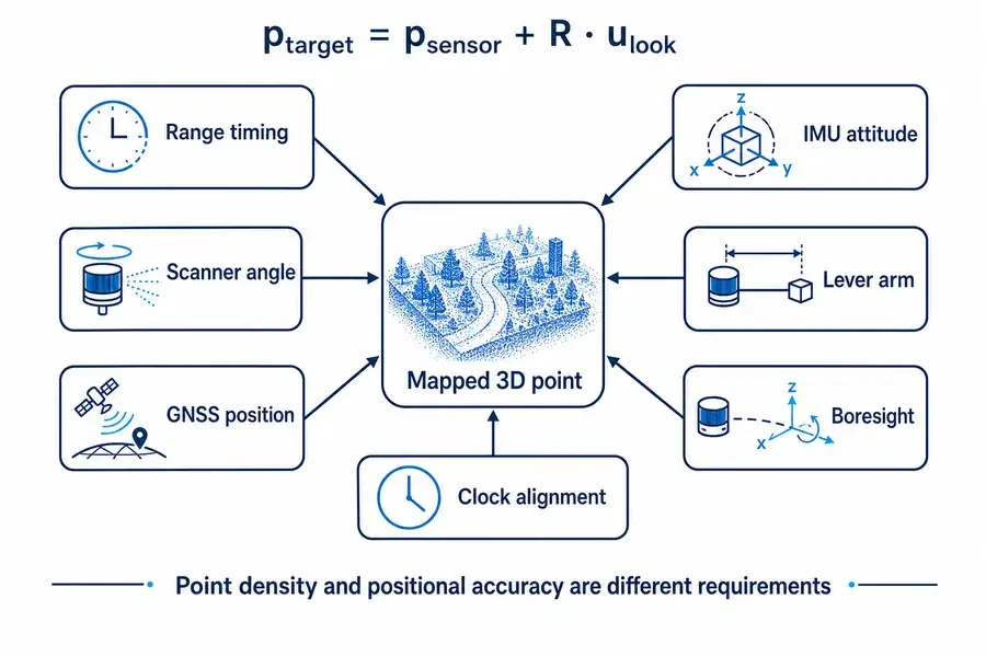
An engineering accuracy budget should separate at least:
- Range error: pulse waveform, detector noise, timing resolution and estimator bias.
- Angular error: scanner encoder accuracy, mirror behavior and optical alignment.
- Position error: GNSS solution quality and antenna placement.
- Attitude error: roll, pitch and heading uncertainty from the inertial system.
- Lever-arm error: uncertainty between the navigation origin and optical reference point.
- Boresight error: angular misalignment between the scanner and navigation frames.
- Time-alignment error: latency and clock offset among the source, scanner, receiver and navigation sensors.
- Calibration and processing error: coordinate transforms, strip adjustment and classification.
Angular and attitude errors grow with distance. For example, an angular error of 0.01° produces roughly 17 cm of transverse displacement at 1 km before other errors are added. This is why absolute mapping accuracy cannot be inferred from the laser pulse width.
Optical and receiver integration
Detector and filter
InGaAs detectors are commonly used for 1.5 µm direct-detection systems. Confirm responsivity at the selected wavelength, active area, gain, bandwidth, excess noise, saturation behavior and temperature dependence. The optical filter should balance background rejection against laser wavelength tolerance, incidence-angle shift and operating-temperature drift.
Beam delivery
Fiber output simplifies routing, but the system still needs a defined connector, mode-field or core specification, numerical aperture, polarization requirement and minimum bend radius. The collimator and scanner aperture set transmitted beam diameter and divergence. Check peak optical intensity at every fiber end face, coating and optical surface.
Receiver field of view
A narrow receiver field of view reduces background light but increases alignment sensitivity. A wider field accepts more angular error and scattered light. Match it to transmit divergence, scanner pointing error, platform vibration and near-to-far operating geometry.
Near-field behavior
Long-range return margin does not guarantee short-range performance. Receiver saturation, optical crosstalk, detector recovery and minimum gate delay can define the minimum usable distance. Test the closest high-reflectivity surface as well as the farthest dark surface.
Electrical, timing, thermal and mechanical integration
External trigger and timing
Define trigger voltage levels, edge polarity, pulse width, input impedance, maximum rate, enable behavior and fault states. More importantly, specify the delay from trigger input to optical emission and its variation over temperature, voltage, repetition rate and unit-to-unit production. Stable latency and low variation reduce calibration burden.
Power architecture
The listed 9–13 V supply range supports compact host designs, but the system engineer should confirm startup current, steady-state power, ripple tolerance, grounding, protection and transient behavior for the chosen operating point. Size cabling and converters for the real pulse mode, not only nominal voltage.
Thermal path
The ambient temperature rating does not define the allowed baseplate temperature in every enclosure. Model heat flow from the laser housing into the host, include solar load and reduced convection where relevant, and validate the hottest sustained pulse program. A stable thermal interface supports repeatable wavelength, timing and optical output.
Mechanical datum and fiber routing
Use a controlled mounting datum, appropriate fastener preload and a protected fiber exit. Avoid forcing the fiber to absorb enclosure tolerance or vibration. Confirm connector access, bend radius, strain relief and service procedure before finalizing the housing.
A qualification plan built around the operating point
An effective source evaluation should reproduce the real system conditions:
| Test | What to record | Why it matters |
|---|---|---|
| Optical output versus repetition rate | waveform, pulse width, peak power and average power | Confirms the usable operating map |
| Timing over temperature | trigger-to-optical delay and variation | Protects range calibration |
| Wavelength and spectral stability | center wavelength and drift | Verifies detector and filter compatibility |
| Long-duration pulse program | output stability, electrical load and case temperature | Exposes thermal limits |
| Low- and high-reflectivity surfaces | detection probability, bias and false returns | Tests real link margin |
| Near- and far-distance scenes | saturation, recovery, ambiguity and missed returns | Validates the full range window |
| Sunlit and low-background conditions | noise floor and detection threshold | Tests background rejection |
| Vibration and routing configuration | optical stability and fiber condition | Validates host integration |
| Point-cloud calibration run | strip alignment, repeatability and absolute checks | Connects source performance to the final deliverable |
Qualification should use the intended detector, optics, scanner timing, navigation sensors and processing chain. A bench power measurement alone cannot qualify a mapping payload.
What to include in your request for quotation
Send these inputs to receive a useful first-pass recommendation:
| Category | Information to provide |
|---|---|
| Application | airborne, mobile, terrestrial, robotic or industrial scanning |
| Scene | surface types, lowest expected reflectivity and environmental conditions |
| Geometry | minimum and maximum distance, altitude or stand-off, field of view |
| Data goal | points per second, point spacing, coverage rate and number of returns |
| Performance | range precision, absolute accuracy and detection probability |
| Timing | repetition-rate range, trigger format, acceptable latency and variation |
| Receiver | detector type, aperture, filter bandwidth and receiver field of view |
| Optical interface | wavelength, connector, fiber and collimated-beam requirements |
| Host constraints | supply, power budget, envelope, mass target and thermal interface |
| Validation | temperature, vibration, service life and production test expectations |
When some inputs are unknown, provide the platform speed, mapping distance, desired point spacing and detector choice first. Those four values are usually enough to identify the highest-risk assumptions.
Frequently asked questions
Is a 1550 nm pulsed fiber laser automatically better for long-range LiDAR?
No. It can be a strong source architecture, but usable range depends on pulse energy, beam divergence, aperture, surface reflectivity, atmosphere, detector performance, background light and detection criteria. Compare complete link budgets at the required operating point.
Does 2 MHz repetition rate mean two million mapped points per second?
Not necessarily. It means up to two million emitted pulses per second at that source setting. Valid point rate depends on return detection and processing, while spatial point density also depends on the scanner and platform motion.
Can the highest peak power be used at the maximum repetition rate?
Do not assume so. Peak power, pulse energy, average power and repetition rate are linked. Confirm the exact combination needed, including pulse width and temperature, before design release.
Which model is best for 3D mapping?
There is no universal best model. The 1.2 kW class source suits compact 1535 nm designs; the 1.6 kW class source supports 1550 nm systems with a higher average-power class; and the 3 kW class source adds per-pulse margin where its pulse width and operating map fit. Receiver and scanner requirements determine the final choice.
Can a Lumexis rangefinder module generate a point cloud?
It can supply distance measurements to a host, but a mapping system must also know the look direction, sensor position, attitude and time for each measurement. Dense scanning generally starts with a pulsed laser source plus a scanner and receiver.
What information is needed to customize a source?
Specify wavelength, repetition-rate range, optical power at the required operating point, pulse width, trigger behavior, fiber or free-space interface, supply, envelope, temperature range and validation conditions. Lumexis can then evaluate optical, electrical and mechanical options.
Build the source around the measurement
A reliable LiDAR design begins with the point cloud, works backward through navigation, timing and detection, and only then fixes the laser operating point. Lumexis supports OEM teams with compact 1.5 µm pulsed sources, engineering communication and configuration review for civil, industrial and research mapping systems.
Discuss your LiDAR laser source requirements with our engineering team.
Please include the intended distance window, point-rate goal, scanner concept, receiver type and host constraints.
Lumexis — precision laser sources, engineered for the real world.
Technical references
- NOAA National Geodetic Survey: What is LIDAR? — point-cloud generation from range, scan angle, position and attitude; topographic and bathymetric wavelength distinction.
- U.S. Geological Survey: What is Lidar Data? — active remote sensing and three-dimensional point-cloud fundamentals.
- U.S. Geological Survey: Lidar Base Specification 2025 Revision A — current topographic data acquisition and quality framework.
- U.S. Geological Survey: Topographic Data Quality Levels — pulse density and vertical positional accuracy as separate quality components.
- Hamamatsu Photonics: InGaAs APD for LiDAR — representative spectral response and 1.5 µm detector context.
- Li et al., Sensors: Influence of Laser Pulse Shape on Ranging Accuracy — effects of pulse shape, signal-to-noise ratio and estimation on time-of-flight ranging.
- Lee et al., Sensors: Pulse Coding for Range Ambiguity Mitigation — pulse-association ambiguity and coding approaches at higher repetition rates.