
Distributed temperature sensing
Distributed Temperature Sensing: Build Around the Fiber
Lumexis develops compact 1550 nm pulsed laser-source configurations for industrial and scientific distributed temperature sensing instruments, with pulse timing, Raman backscatter collection, calibration, fiber length, and the host acquisition chain reviewed as one system.

Match the thermal-monitoring task before selecting the laser
Distributed temperature sensing turns an optical fiber into a continuous line of temperature measurement points. For power cables, tunnels, conveyors, utility pipelines and environmental research, this can reveal where a thermal change occurs—not only whether one discrete sensor crossed a threshold.
Lumexis develops configurable 1550 nm pulsed fiber laser sources for Raman optical time-domain reflectometry systems. The source platform combines adjustable nanosecond pulses, low average optical power, internal or external triggering and fiber output for integration into an OEM DTS interrogator.
This solution is a strong starting point when the system team needs:
- a 1550 nm source for a Raman-OTDR architecture;
- adjustable 1–20 ns pulse width;
- adjustable 5–200 kHz repetition frequency;
- up to 50 W peak-power capability at a qualified operating point;
- low average optical power for a sensitive backscatter receiver;
- synchronized acquisition through internal or external triggering;
- an FC/APC fiber interface and an option to integrate the Raman WDM.
It is not a complete DTS instrument. Measuring distance, spatial resolution, temperature accuracy, update time and alarm performance depend on the laser, sensing fiber, Raman filters, detectors, timing electronics, calibration and processing as one system.
Fast selection rule: Begin with sensing-fiber length and required spatial detail. Use those inputs to set pulse width and repetition rate, then close the Raman return, receiver-noise, timing and thermal budgets at one achievable laser operating point.
Where distributed fiber temperature monitoring fits
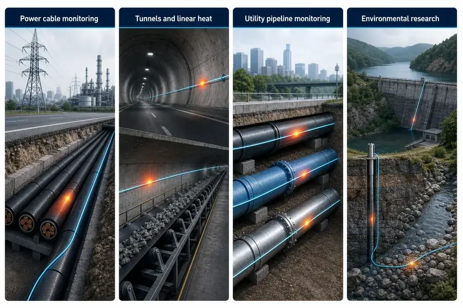
Application fit
Match the optical source to the real measurement task
Four Distributed Temperature Sensing application classes: power cables, tunnels and conveyors, utility pipelines, and environmental research
Power cable and electrical infrastructure monitoring
A sensing cable installed beside an underground, subsea or industrial power cable can provide a continuous temperature profile along the route. System software may then identify local hot sections, compare circuits and support thermal-condition assessment. Source selection should reflect route length, required localization, cable loss, splice count and the update time needed by the monitoring logic.
Tunnels, conveyors and linear heat monitoring
Road and rail tunnels, conveyor corridors, cable trays and long industrial spaces are difficult to cover with isolated point sensors alone. DTS can localize abnormal heating along the fiber and provide rate-of-rise information to the host monitoring platform. Alarm design, coverage rules and final system compliance remain responsibilities of the complete installation.
Utility and process pipelines
Temperature profiles can support monitoring of district-heating lines, water systems and industrial utility pipelines. The value comes from correlating a thermal anomaly with its distance along the cable. The fiber placement and thermal coupling to the asset are just as important as interrogator performance.
Dams, boreholes and environmental research
Fiber-optic temperature data can reveal groundwater exchange, seepage, flow paths and thermal changes in boreholes or along streambeds. These measurements often prioritize calibration quality and long-term stability over rapid alarms. Single-ended and double-ended layouts should be considered before the cable is installed.
Industrial process and scientific instruments
Kilns, storage areas, test structures and research installations can benefit from many temperature samples without placing electrical sensors at every location. The correct sensing cable and installation method must match the temperature range, chemical exposure, bend requirements and desired thermal response.
When DTS is not the natural first choice
An application may be better served by another sensing architecture when:
- only one or two accessible temperature points are required;
- millimeter-scale local detail matters more than long continuous coverage;
- the measurement must separate strain and temperature without additional compensation;
- the sensing fiber cannot be thermally coupled to the object or medium;
- installation access, connector loss or cable repair makes a continuous fiber route impractical;
- the required response is faster than the available Raman signal averaging allows.
DTS should also not be confused with distributed acoustic sensing. Raman DTS is designed to estimate temperature from inelastic backscatter intensity, while acoustic systems usually analyze coherent Rayleigh backscatter and require a different laser and receiver architecture.
The Lumexis DTS laser-source configuration
The following values are for initial engineering matching. They are source specifications, not complete DTS-system performance claims.
| Parameter | Current configuration | Why it matters in Raman DTS |
|---|---|---|
| Operating mode | Pulsed | Provides time-of-flight location along the sensing fiber |
| Center wavelength | 1550 nm typical; 1547–1553 nm range | Must match Raman WDM passbands, detector response and fiber design |
| Pulse width, FWHM | 1–20 ns adjustable; 3 ns typical | Contributes to spatial resolution and pulse energy |
| Repetition frequency | 5–200 kHz adjustable; 10 kHz typical | Sets the available return window and affects averaging speed |
| Spectral width | 0.5 nm typical at 3 dB | Influences filter matching and spectral separation |
| Average optical power | 2 mW typical; 3 mW maximum | Connects pulse energy, repetition rate and thermal/electrical load |
| Peak power | Up to 50 W | Contributes to Raman return margin at the selected operating point |
| Timing jitter | 0.3 ns maximum | Supports stable range-to-position registration |
| Triggering | Internal or external | Enables synchronization with acquisition electronics |
| Optical interface | FC/APC patch cord | Supports fiber-coupled OEM integration |
| Raman WDM | Integration option | Can reduce optical-front-end integration work |
| Supply | 12 V nominal | Supports compact instrument power architecture |
| Power consumption | 3 W maximum | Helps size the electrical and thermal design |
| Operating temperature | −20 to +60 °C | Defines the source qualification envelope |
| Storage temperature | −40 to +85 °C | Supports transport and non-operating design checks |
| Package | 150 × 120 × 21 mm | Defines enclosure and mounting space |
| Weight | 500 g maximum | Supports instrument mechanical budgeting |
The wavelength, pulse width, repetition rate, peak power and average power must be specified together. Do not assume every maximum in the table can occur simultaneously.
How Raman DTS converts time and backscatter into temperature
System architecture
Review the complete optical and measurement chain
Typical Raman OTDR system chain from a pulsed laser source and sensing fiber to Stokes and anti-Stokes detectors and a temperature profile
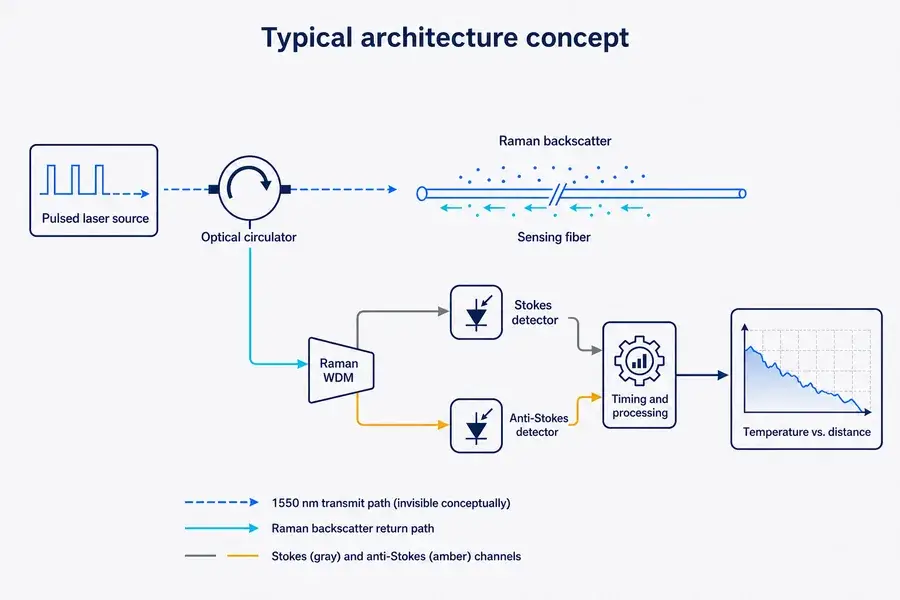
A typical Raman-OTDR interrogator launches a short optical pulse into the sensing fiber. A small fraction of the light is scattered back toward the instrument. The return time provides distance:
z = vgΔt / 2
where (z) is position along the fiber, (v_g) is the group velocity in the fiber and (Δ t) is the round-trip delay.
The optical front end separates two Raman-shifted bands:
- Stokes: shifted to a longer wavelength than the launch light and comparatively less temperature sensitive.
- Anti-Stokes: shifted to a shorter wavelength and strongly dependent on the local thermal population of the glass.
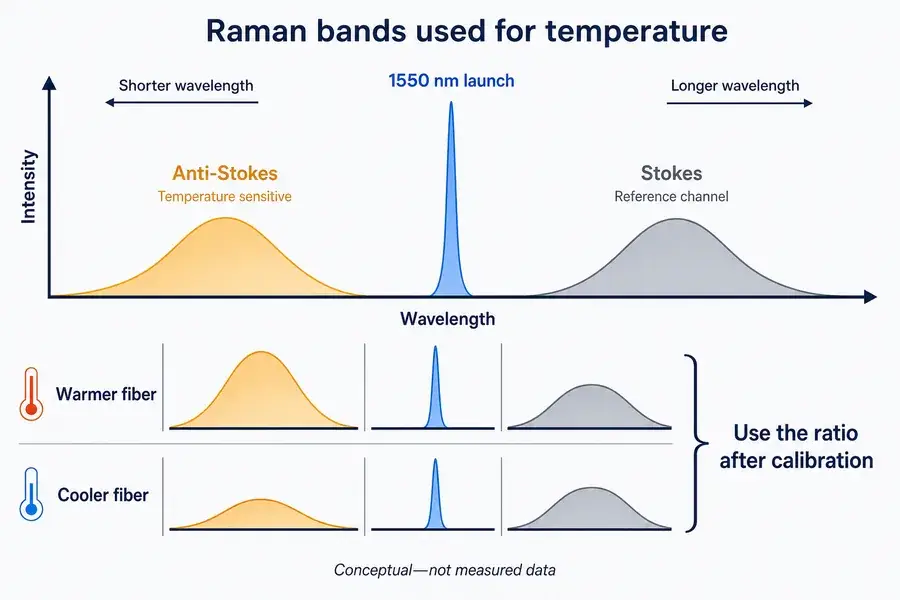
Engineering visual
See how the source fits the complete instrument
Conceptual Raman spectrum showing anti-Stokes, a 1550 nm launch peak, Stokes and the warmer-versus-cooler intensity relationship
Temperature is derived from the ratio of the received Stokes and anti-Stokes powers after instrument and fiber calibration. One commonly used form is:
T(z,t) = γ / [ln(PS/PAS) + C(t) − ∫0zΔα(z′)dz′]
Here, (P_S) and (PAS) are the received Stokes and anti-Stokes powers, (γ) contains the Raman energy-shift term, (C(t)) represents instrument calibration, and (Δα) is the differential attenuation between the two Raman bands.
This equation explains an important procurement boundary: a stable pulse source is necessary, but absolute temperature quality also depends on spectral filtering, receiver response, connector and splice loss, cable condition and calibration.
Select the source from four coupled laser parameters
Parameter interaction
Evaluate coupled parameters at the operating point
DTS laser source selection diagram relating pulse width, pulse energy, repetition rate, timing jitter and ASE noise to system behavior
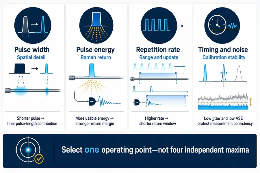
Pulse width controls the pulse-length contribution to spatial detail
For a first-pass calculation:
Δzpulse ≈ vgτp / 2
Using a representative group velocity of approximately (2.0×10^8) m/s:
| Pulse width | Ideal pulse-length contribution |
|---|---|
| 1 ns | approximately 0.10 m |
| 3 ns | approximately 0.30 m |
| 10 ns | approximately 1.0 m |
| 20 ns | approximately 2.0 m |
These are not guaranteed DTS spatial-resolution values. Detector bandwidth, sampling rate, fiber modal dispersion, filtering and the definition used for the 10–90% response all broaden the system result. A shorter pulse also carries less energy if peak power is unchanged, so spatial detail and Raman return margin must be balanced.
Pulse energy drives usable Raman return
The energy in one pulse is:
Ep = ∫P(t)dt
For an ideal rectangular pulse, (E_p≈ Ppeakτ_p). A 50 W, 3 ns rectangular pulse would contain approximately 0.15 µJ. The real value must be calculated from the measured waveform; it should not be treated as a guaranteed product figure.
More pulse energy can improve the very weak Raman return, but excessive launched power can increase nonlinear effects, receiver recovery demands, back-reflection stress and unwanted optical background. Return margin should be evaluated with the actual fiber, WDM, detector and acquisition bandwidth.
Repetition rate sets the available return window
The next pulse should not be confused with the return from the previous pulse. For simple uncoded operation, a first-pass unambiguous sensing length is:
Lunamb ≈ vg / (2frep)
Using (v_g≈2.0×10^8) m/s:
| Repetition frequency | Simple first-pass return window |
|---|---|
| 5 kHz | approximately 20 km |
| 10 kHz | approximately 10 km |
| 50 kHz | approximately 2 km |
| 200 kHz | approximately 0.5 km |
This table is not a product measuring-distance claim. Coded sequences, gating and other correlation methods can change the architecture, while fiber attenuation and Raman signal-to-noise ratio may limit practical distance before ambiguity does.
Average power closes the operating point
Average optical power connects energy and pulse rate:
Pavg = Epfrep
For example, the ideal 0.15 µJ pulse above at 10 kHz gives 1.5 mW average optical power. The calculation is consistent with the scale of the current source configuration, but actual output must be confirmed from the qualified waveform and operating map.
This is why peak power, pulse width and repetition rate cannot be purchased as three independent maxima. Lumexis should confirm the exact combination required by the interrogator.
Timing jitter and ASE set a quieter measurement foundation
Timing variation shifts the apparent position of a return. In a fiber with group velocity near (2.0×10^8) m/s, 0.3 ns corresponds to about 3 cm of one-way position contribution before sampling and other errors are considered.
Amplified spontaneous emission and other source background can enter the receiver passbands or reduce available dynamic range. System teams should therefore review time-resolved waveform quality, extinction between pulses, spectral background, back-reflection behavior and power stability—not only the pulse peak.
Wavelength and Raman WDM integration
A 1550 nm launch wavelength can support compact fiber components and OEM architectures, but the source cannot be selected independently from the receiver.
Confirm:
- the exact Stokes and anti-Stokes center wavelengths created by the fiber’s Raman shift;
- Raman WDM passbands, isolation and insertion loss;
- detector responsivity and noise at both return bands;
- suppression of the 1550 nm Rayleigh and residual launch light;
- spectral drift over the complete operating temperature;
- connector cleanliness, back reflection and return loss;
- sensing-fiber type, core size, numerical aperture and modal behavior.
The optional integrated Raman WDM can reduce packaging and alignment work, but its ports, spectral bands and isolation should be specified against the intended detectors and sensing fiber.
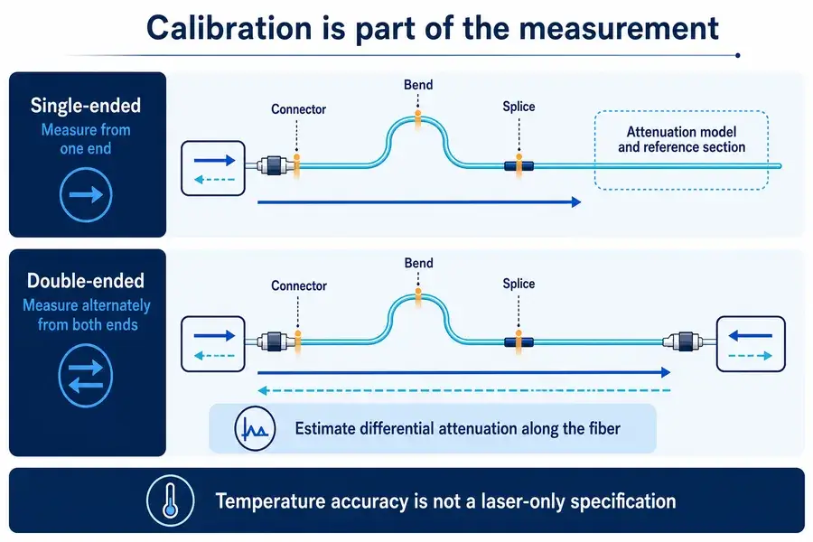
Temperature accuracy is a calibration-chain result
Accuracy chain
Treat accuracy as a complete calibration result
Single-ended and double-ended DTS calibration diagram showing connector, bend and splice losses and differential-attenuation correction
Single-ended measurement
The interrogator launches and receives from one end of the cable. This is simpler to install, but the temperature calculation needs an attenuation model and one or more known-temperature reference sections. Local bends, connectors and splices can change the differential loss between Raman bands and appear as false temperature offsets if they are not corrected.
Double-ended measurement
The system measures the same fiber alternately from both ends. Combining both directions allows position-dependent differential attenuation to be estimated more directly. This can improve field calibration, particularly along non-uniform or spliced cables, but requires a looped fiber path, additional switching or channels and more processing.
Keep these performance terms separate
- Sampling interval: distance between reported data samples.
- Spatial resolution: physical length needed to resolve a temperature transition.
- Temperature resolution: smallest detectable temperature change under stated conditions.
- Temperature accuracy: closeness to the calibrated reference temperature.
- Repeatability: variation when the same condition is measured again.
- Measurement time: integration and processing time needed for one profile.
These values are related but not interchangeable. A fine sampling interval does not prove equally fine spatial resolution, and a stable laser does not by itself establish system temperature accuracy.
Optical, electrical and mechanical integration checklist
Optical path
- Confirm FC/APC interface, fiber type and maximum allowed back reflection.
- Define whether the Raman WDM is inside the source package or in the host optical module.
- Specify launch isolation, receiver protection and any required monitor channel.
- Test connectors, bends and splices representative of the installed sensing cable.
Trigger and acquisition
- Define internal or external trigger mode and switching behavior.
- Specify trigger voltage, polarity, pulse width and input impedance.
- Measure trigger-to-optical delay and its variation with temperature and pulse settings.
- Synchronize the ADC window with the full round-trip time of the sensing fiber.
Electrical and thermal design
- Confirm startup, steady-state and transient current at 12 V.
- Provide a controlled mounting surface and conductive heat path.
- Validate the longest sustained pulse program at the hottest baseplate condition.
- Check grounding and isolation between the laser driver, detector front end and data acquisition.
Mechanical layout
- Reserve the 150 × 120 × 21 mm source envelope plus connector and fiber-bend clearance.
- Protect the FC/APC patch cord from tension, sharp bends and enclosure tolerances.
- Place service connectors where cleaning and inspection can be performed without stressing the fiber.
- Define shock and vibration requirements from the actual host instrument.
Qualification should reproduce the final DTS operating point
| Test | Record | System question answered |
|---|---|---|
| Output versus pulse settings | waveform, pulse width, peak and average power | Which combinations are actually available? |
| Timing versus temperature | trigger delay and jitter | Will position registration remain stable? |
| Spectrum versus temperature | center wavelength, width and background | Will the Raman WDM and detector bands stay aligned? |
| Long-duration operation | case temperature, output stability and power draw | Can the host sustain the intended measurement cycle? |
| Back-reflection test | output recovery, faults and stability | Will the source tolerate the optical network? |
| Fiber-length test | return window and trace overlap | Is the selected repetition rate appropriate? |
| Receiver-background test | noise floor with and without launch | Is ASE or leakage consuming dynamic range? |
| Calibrated temperature sections | bias, repeatability and uncertainty | Does the full interrogator meet the measurement goal? |
| Connectors, bends and splices | local loss and false offsets | Is field installation represented? |
Bench-testing the laser separately is necessary, but final qualification must include the Raman WDM, detectors, sensing cable, calibration sections and processing software.
What to include in a DTS laser-source RFQ
| Category | Information to provide |
|---|---|
| Application | power cable, tunnel, conveyor, utility pipeline, borehole, dam or research instrument |
| Fiber route | total optical length, single- or double-ended layout, splice and connector count |
| Sensing fiber | single-mode or multimode, core size, numerical aperture and cable construction |
| Spatial requirement | required localization, sampling interval and spatial resolution definition |
| Thermal requirement | temperature range, required accuracy, resolution and response time |
| Measurement cycle | profile update time, averaging time and duty cycle |
| Laser operating point | wavelength, pulse width, repetition rate, pulse energy or peak power |
| Receiver | Raman WDM bands, detector type, bandwidth, gain and saturation limit |
| Timing | internal or external trigger, acceptable delay and jitter |
| Host constraints | supply, power budget, envelope, mass and cooling surface |
| Environment | operating temperature, vibration, humidity and cable exposure |
| Production | annual volume, validation plan and traceability requirements |
When the receiver is not yet fixed, send the sensing-fiber length, required spatial resolution, update time and preferred detector bands first. Those inputs expose the main architecture tradeoffs.
Frequently asked questions
What is Distributed Temperature Sensing?
Distributed Temperature Sensing is a fiber-optic measurement method that reports temperature as a function of distance along a sensing cable. In Raman DTS, a pulsed laser and time-resolved Stokes/anti-Stokes backscatter measurement create the temperature profile.
Why use a pulsed laser instead of a continuous source?
The pulse provides a time reference. Because the return delay increases with distance along the fiber, the interrogator can associate Raman backscatter with position.
Is the Stokes or anti-Stokes signal temperature sensitive?
The anti-Stokes band has the stronger temperature dependence. Many Raman DTS systems use the ratio of anti-Stokes and Stokes signals so the Stokes channel helps normalize source and path effects. Calibration is still required.
Does a 1 ns laser pulse guarantee 10 cm DTS spatial resolution?
No. About 10 cm is the ideal pulse-length contribution in fiber. Detector bandwidth, acquisition, dispersion, filtering and response-definition methods broaden the system result.
Can 200 kHz be used on a 20 km sensing fiber?
Not with a simple one-pulse-at-a-time return window. At 200 kHz, the first-pass unambiguous length is approximately 0.5 km. Long fibers normally require a lower rate or a deliberately coded/correlated architecture.
Does 50 W peak power determine the measuring distance?
No. Practical range depends on pulse energy, fiber loss, Raman backscatter, WDM insertion loss and isolation, detector noise, averaging time and required temperature uncertainty. The 50 W value is a source ceiling at a qualified operating point, not a DTS range specification.
Can the Raman WDM be integrated into the laser source?
The present configuration can support Raman WDM integration. Final passbands, isolation, connector arrangement and detector compatibility must be defined for the interrogator.
What determines DTS temperature accuracy?
The Raman signal ratio, instrument drift, detector response, differential attenuation, reference sections, fiber installation and calibration method all contribute. Temperature accuracy is a complete-system specification.
Build the source around the sensing fiber
The most reliable DTS projects start with cable length, spatial detail, update time and calibration method. Those requirements define the pulse operating point and receiver architecture more effectively than selecting the largest peak-power value.
Lumexis works with OEM instrument teams to configure 1550 nm pulsed fiber laser sources, triggering, fiber interfaces and Raman optical integration for civil, industrial and scientific distributed temperature sensing.
Discuss your DTS laser-source requirements with our engineering team.
Please include sensing-fiber length, target spatial resolution, profile update time, Raman WDM bands and host constraints.
Lumexis — precision laser sources, engineered for the real world.
Technical references
- U.S. Environmental Protection Agency: Fiber Optic Distributed Temperature Sensing — Raman backscatter, Stokes/anti-Stokes ratio, time-to-distance mapping, calibration and environmental applications.
- van de Giesen et al.: Double-Ended Calibration of Fiber-Optic Raman Spectra DTS Data — Raman temperature equation, differential attenuation and single-/double-ended calibration.
- National Institute of Standards and Technology: High-Resolution Distributed Raman Sensor — 1550 nm Raman sensing and the relationship among source, detector and spatial performance.
- Ukil, Braendle and Krippner: Distributed Temperature Sensing—Review of Technology and Applications — DTS technology families, system principles and application context.
- U.S. Department of Energy OSTI: Design and Implementation of Distributed Raman Temperature Sensing — laser wavelength, pulse width, spatial resolution and receiver design tradeoffs.
- Tyler et al.: Environmental Temperature Sensing Using Raman Spectra DTS — field deployment, calibration and environmental measurement context.
- Li et al.: High-Temperature Raman DTS with Different Special Fibers — representative Raman-OTDR architecture and pulse-width/spatial-resolution example.